The following text is a detailed summary of my PhD topic. More details can be found in the accompanying dissertation.

 

Introduction

The classification of pathological changes in the structure and function of the human body are daily tasks in medicine. In many cases, the decision for a class is based on the physician's knowledge and experience and is therefore rather subjective. Motivated by this fact, guidelines and regulations for classification based on hard metrics and quantitative measures are becoming prevalent. This methodology ensures more objective and reproducible choices with less intra-, and inter-rater variability. Most recently, the fully automatic processing of medical data by methods of pattern recognition has begun to emerge.

Additionally, it is a well supported fact that data stemming from multiple modalities can improve the diagnostic performance of manual as well as of automatic classification schemes.

 

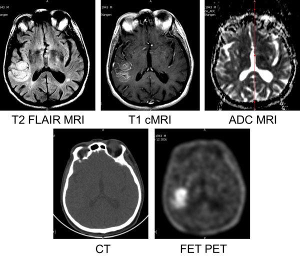
Figure 1: Multimodal images of a 68 year old, male patient, diagnosed with Glioblastoma (WHO4) by biopsy.

 

Cerebral gliomas are a common type of cancer with a incidence of 6 per 100000 individuals per year in Germany (1). The most common subtypes of gliomas are glioblastoma (54%) and other astrocytomas (22%). Another subtype are oligodendrogliomas. The different subtypes are subject to different treatments in clinical routine, which is reflected in the guidelines for the diagnosis and treatment of this tumour entity (1). The differentiation between these subtypes, namely the classification of the tumour on basis of medical images and bioptic samples, is an important and challenging task. The gold standard in terms of diagnostic confidence is the grading of the tumour based on histologic analysis of invasively gained bioptic samples. The bioptic grading allows an accurate classification in over 90% of all cases (1). However, the process of taking the bioptic samples, whether stereotactic, incisional, or excisional biopsies, in general results in an increased risk for complications during the surgery. This is reflected by a reported morbidity ranging from 5-9% (2, 3) for stereotactic biopsies. Statistics such as these motivate the desire for accurate non-invasive grading.

It is generally accepted that MRI of the human brain is the standard for an initial diagnosis of glial tumours. A variety of different MRI sequences are acquired to cover different aspects of the tumour. Nevertheless, other imaging modalities like e.g. X-ray CT and PET using FET can add beneficial information for the task of tumour grading. In the end, it is common that, for each patient, more than 5 to 10 3-D medical datasets from different modalities at various time points exist, each covering the same anatomical structures. This results in increased complexity for the physician who must diagnose and classify using the multitude of images.

Automatic classification approaches promise the ability to overcome the limitations of human beings, by providing classification on high-dimensional data based on objective measures/features.

The aim of this study is to evaluate the classification accuracy of different automatic classifiers of PET, CT and MRI data of cerebral gliomas and to elaborate the potential benefits of this multimodal approach.

Material and Methods

An initial screening of patients examined with FET-PET/CT in the Clinic of Nuclear Medicine in Erlangen yielded 232 patients between 05-Jun-2007 and 21-Mar-2011. After applying our inclusion criteria (listed below), 16 patients remained. 32 patients from the Institute of Neuroscience and Medicine at Forschungszentrum Jülich also met the criteria and were included in our analysis. Table 1 provides additional details like age, weight, injected dose, time between the acquisition and several other parameters of the patient population.

 

Inclusion criteria:

• Dynamic PET acquisition using the amino acid FET, optional: CT images
• T2-weighted MRI, contrast-enhanced T1-weighted MRI, optional: diffusion-weighted MRI
• No prior treatment (esp. surgery, chemotherapy, radiotherapy)
• After imaging: Tumour classification by histology on bioptic sample

As we had two different classification tasks, the differentiation between low and high-grade and the differentiation between the individual WHO grades, we created different (overlapping) subsets of our patient population for each tasks. The set SUB44 consisted of the T1-MRI, T2-MRI and dynamic PET data of 44 patients (22 low grade, 22 high grade). SUB32 consisted of the T1-MRI, T2-MRI and dynamic PET data of 32 patients (8 WHO1, 8 WHO2, 8 WHO3, and 8 WHO4). SUB22 consisted of ADC-MRI data of 22 patients (11 low grade, 11 high grade). SUB14 consisted of the CT data of 14 patients (7 low grade, 7 high grade). For all subsets, the number of patients in each class was balanced by random sampling.

 

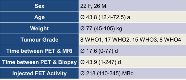
Table 1: Parameters of the patient population

 

Image Acquisition

The image acquisition consisted of two main procedures for all patients in our collective. One is the PET(/CT), the other the MRI. The details of the acquisitions are described in the corresponding sections.

CT

After the patient positioning, a low-dose CT scan was acquired. The following parameters were chosen: Size of the focal spot: 1.2 mm; Rotation time: 1.0 s; Tube voltage: 120 kV. The actual mean current for our patient collective was approximately 50 mAs. We reconstructed 2 datasets using the manufacturer-supplied FBP methods, one with a softer kernel (B08s) for attenuation correction purposes, and one with a sharper kernel (B41s) for automatic classification and reading by the physicians. Both datasets had a matrix size of 512x512x111 (0.49x0.49x2.00 mm). The image intensities were in Hounsfield Units (HU). After the CT procedure, the patient is transferred to the PET part of the gantry by an automatic table movement in axial direction.

PET

The PET & CT data for 16 patients were acquired using a hybrid PET/CT system (TruePoint Biograph 64, Siemens Healthcare MI). The PET and the CT were integrated into a common gantry in sequential spatial order. The PET data for the remainder of the patients (32) were acquired on the ECAT EXACT HR+ (Siemens Healthcare MI).

The TruePoint Biograph 64 system is equipped with Lutetium Oxyorthosilicate (LSO) as detector material. Each detector block consists of 13x13=169 individual detector elements, each with the size 4.0x4.0x20 mm. Our scanner had 4 detector block rings, each consisting of 48 detector blocks. This resulted in a total number of 32448 detector elements. The transaxial FOV was 605 mm, the axial 216 mm. According to the manufacturer, the axial resolution was 5.7 mm, and the transaxial resolution was 4.8 mm at 10 cm distance from the centre of the FOV, measured using the NEMA 2001 standard.

The other scanner used for our study was the ECAT EXACT HR+. It is equipped with Bismuth Germanate (BGO) as scintillator material and each detector block consisted of 8x8=64 individual detector elements, each with the size 4.0x4.4x30 mm. It had 4 detector block rings, each consisting of 72 detector blocks. The total number of detector elements subsequently was 18432. The transaxial FOV was 155 mm, the axial FOV was 583 mm. The axial resolution was 5.3 mm, the transaxial resolution 5.4 mm at 10 cm distance to the centre of the FOV. The ECAT EXACT HR+ is no hybrid device, and instead uses three Ge-68/Ga-68 rod sources to acquire transmission data for attenuation correction.

The PET acquisition started simultaneously with the injection of the radioactive tracer. The PET images were acquired over 40-50 minutes, the raw PET detector events were recorded together with a time stamp (listmode acquisition). This allowed a retrospective reconstruction into any desired combination of time bins. For the Biograph 64, we choose 5 short (1 minute each)  bins at the beginning of the acquisition and subsequently 7 long (5 minutes each) time bins throughout the end of the acquisition (40 minutes total). The time bins for the ECAT EXACT HR+ varied slightly (5x1 minute, 5x3, 4x5 or 6x5 minutes (40/50 minutes total). The raw data of each bin were reconstructed into (nearly) isotropic 3-D datasets with a matrix size of 168x168x109 (2.03x2.03x2.02 mm), using the iterative OSEM algorithm with 6 iterations and 8 subsets and CT based attenuation correction for the Biograph 64 and 128x128x63 (2.00x2.00x2.42 mm) with either FBP (Shepp-Logan Filter FWHM 2.48 mm) or iterative OSEM with 6 iterations and 16 subsets and Ge-68/Ga-68 transmission based attenuation correction for the ECAT EXACT HR+. Corrections for decay, scatter and random coincidences were applied for both scanners according to the implementation of the manufacturer. For the Biograph 64, smoothing with a Gauss filter (Kernel width 5 mm) was used as post-processing step. Consequently, this yielded in total 12 3-D datasets from the Biograph 64 and 14 or 16 3-D datasets from the ECAT scanner. As both PET scanners were calibrated in order to allow absolute quantification, the image intensities were in Becquerel per Millilitre.

MRI

The MRI acquisitions were done on various systems: One Philips 1.0 T system (Gyroscan NT),  three Siemens 1.5 T systems (Magnetom Avanto, Magnetom Sonata, Magnetom Symphony, Siemens Healthcare, Erlangen), one Philips 1.5 T system (Intera, Philips Electronics N.V.) and one 3 T system (Magnetom Trio, Siemens Healthcare).

 

T1-MRI

For the T1-weighted MRIs, an intravenous injection of 0.1 mmol/kg  body weight Gadobutrol (Gadovist, Bayer Schering Pharma) was used in most cases as contrast agent (alternatively Gadodiamide, Omniscan, GE Healthcare; Gadopentetate dimeglumine, Magnevist, Bayer Schering Pharma). The images were acquired with a TE ranging from 1.7 to 17 ms and TR ranging from 145 to 690 ms. The typical slice thickness was 3-6 mm with an in-plane pixel size of 0.4-0.9 mm. However, the parameters for the (almost) isotropic T1-MRI (MPRAGE) differed: The TE was 2.2-3.93 ms, TI was 900-1100 ms, TR was 1950-2200 ms, in plane pixel size was 0.5-1.1 mm with 1.0-1.5 mm slice thickness.

 

T2-Flair MRI

The anisotropic T2-Flair MRIs were acquired using an inversion time of 1800-2500 ms, TE ranged 79-150 ms, TR 5000-10000 ms. The in-plane pixel size was 0.4-1.0 mm with a slice thickness of 3-6 mm. Again, the parameters for the isotropic datasets differed: The TI was 1800 ms, TE was 389 ms, TR was 5000 ms. The in-plane pixel size was 0.5 mm and the slice thickness was 1 mm.

 

ADC MRI

For the diffusion weighted MRIs, the TE was 91-101 ms, TR was 3200-3900 ms. The in-plane pixel size was 0.6-1.8 mm and the slice thickness ranged 5-6 mm.

Volume of Interest Definition

In general, it is possible to define a VOI in several ways: There exist fully automatic (e.g. by automatic segmentation), semi-automatic (by segmentation using manually defined seed points) and manual methods.

We decided to use a manual delineation of the VOI on the basis of the images from T2-weighted MRI. This is motivated by the fact that an implementation and evaluation of the automated methods was beyond the scope of this work. The manual segmentation is known to be robust, enabling us to focus on the classification task itself. In the future, automated methods should be considered as a viable step towards further automation.

The T2-weighted MRI itself is considered as the standard sequence for the tumour localization in the brain. It has a superior soft-tissue contrast when compared to X-ray CT. T2-MRI also promises increased sensitivity and specificity over FET-PET for detecting intracranial lesions. This is mainly caused by the lower spatial resolution of PET when compared to MRI and due to non-specific FET uptake of healthy structures in the brain, which is especially given for tumours that are small and show low FET uptake.

The borders of the tumours were delineated slice-by-slice with help of the ITK-Snap tool by a board-certified radiologist. In addition to the tumour VOI, one contra-lateral, healthy reference VOI with approximately the same volume as the tumour VOI was drawn. An example of this procedure is given in Figure 2.

 

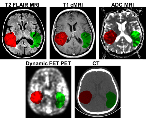
Figure 2: Example for a volume of interest in multimodal images of a 68 year old, male patient, diagnosed with Glioblastoma (WHO4) by biopsy. The red VOI covers the tumour, the green VOI a contralateral, healthy reference region.

 

Due to the heterogeneity of the T2-FLAIR MRI sequences on the different scanners, the image windowing for drawing the VOIs had to be adjusted manually to ensure proper tumour visualization.

The average volume for the tumour and reference VOI were 42.6 cm³, ranging from 2.8 cm³ to 156 cm³. The VOIs were subsequently saved as DICOM datasets and imported into the InSpace volume renderer. Further computations such as co-registration, inter-dataset normalization and feature extraction and calculation were carried out in that program. InSpace is a standalone version of the commercially available Syngo InSpace application (Siemens Healthcare).

Image Registration

The image registration was a crucial part of our workflow. The medical images from different modalities, acquired at different points in time usually did not have an identical intrinsic orientation. This means that a voxel with certain coordinates did not necessarily contain the same anatomical structure of a voxel with the same coordinates in another dataset. The coordinate transformation from the voxel in one dataset to the corresponding voxel in another dataset was in our case obtained by application of a fully automated rigid registration approach.

The registration of the images was carried out using an InSpace plugin. The dataset which was used to define the VOIs (in our case the T2-weighted MRI) was considered as the reference volume. Subsequently, all other datasets were registered to this dataset using a plugin which is based on the algorithms of Hahn et al. (4). The registration itself is realized as a rigid registration and therefore had 6 degrees of freedom (3 translations, 3 rotations). It is based on the pixel intensities of the images and the normalized mutual information is used in its objective function. The objective function is iteratively optimized by a hill climbing algorithm. The algorithm features a multi-resolution approach in order to speed up computational time. More details on the algorithm can be found in (4). We evaluated the accuracy of the retrospective registration between cranial PET and MRI in earlier work (5). We found the registration accuracy to be sufficient for our purpose.

Data Extraction and Feature Calculation

Depending on the modalities included in the classification task, the number of extracted features varied. The nature of the features can be described as statistical, contextual or textural. Statistical means in this context that the feature was calculated on the basis of the intensity value distribution of a single VOI. Contextual means that the feature was calculated by combining features from more than one VOI. In our case this always referred to a combination of the tumour VOI and the reference VOI of a patient dataset. In our implementation, based on the work of Haralick et al. (6), textural features incorporate information about the co-occurrence of intensity values in a VOI. For that reason, grey-level co-occurrence matrices need to be calculated.

We calculated 19 features for every MRI and CT sequence and along with 12 features for the dynamic PET.

Some examples for these features are:

• Mean, maximum, and minimum intensity values in the tumour VOI
• Proportion of hyper-intense voxels in the tumour VOI
• Quotient of the maximum intensity value in the tumour VOI to the mean intensity value in the reference VOI
• Slope and intercept of the time-activity curve in the tumour VOI of the dynamic PET
• Texture energy
• …

Feature Normalization

We applied two different feature normalization methods: Linear scaling to a range and linear scaling to unit variance.

 

Linear Scaling to Range (LSR)

As the different modalities have different image intensity levels and the features have differing numerical ranges, normalization is crucial to ensure that the features are inherently equally weighted. One of the most frequently proposed methods for feature normalization is scaling the features to the interval $[-1;1]$. The training set $\mathcal{S}$ consists of $N$ instances $\mathcal{S}=\left\{(\vec{x}_i,y_i)\right\} \quad i=1,\ldots,N$, with $\vec{x}_i \in \mathbb{R}^{d}$ and $y_{i} \in \mathbb{Z}$. $x_{i,j}$ denotes the $j$-th element of sample $\vec{x}_{i}$. By applying Equation 1 to the $x_{i,j}$ we obtained the normalized values $\tilde{x}_{i,j}$. $\max_j$ and $\min_j$ represent the maximum and minimum values of the $j$-th dimension in the feature set.

$$\tilde{x}_{i,j} = \dfrac{x_{i,j} - \frac{1}{2}(\max_{j} + \min_{j})}{\frac{1}{2}(\max_{j} - \min_{j})} \qquad i=1,\ldots,N, \: j=1,\ldots,d \qquad \text{Eq. 1}$$

Linear Scaling to Unit Variance (LSUV)

As an alternative to scaling to a specified range, scaling to unit variance can be used to ensure an equal weight of all features during the classification process. Scaling to unit variance does not rely on (potentially noisy) extremal values like, e.\,g.\ maxima, minima but on the mean $\mu_{j}$ and the standard deviation $\sigma_{j}$ of $j$-th dimension. We chose to scale the feature values in such a way that for the transformed features $\tilde{\vec{x}}_{i}$, $\tilde{\mu}_{j}=0$ and $\tilde{\sigma}_{j}^{2}=1$. This is achieved using Equation 2 on the values. As previously, $x_{i,j}$ denotes the $j$-th element of sample $\vec{x}_{i}$:

$$\tilde{x}_{i,j} = \dfrac{x_{i,j} - \mu_{j}}{\sigma_{j}} \qquad i=1,\ldots,N, \: j=1,\ldots,d \qquad \text{Eq. 2}$$

In the following, we report the highest classification rates for both normalization methods as we found the difference between the results to be minor.

Feature Selection

Most features were extracted for different modalities, e.g. the Mean Intensity Value of the tumour VOI was extracted for T1-MRI, T2-MRI, ADC-MRI and CT. These one dimensional features were collected into feature sets, according to manually defined rules. The feature sets themselves were one-dimensional if only one feature was included and were of higher dimension if multiple features were included. E.g. one feature set consisted of the six one-dimensional texture features for each modality. Some feature sets contained the transformed features: These were features consisting of a varying component number of the PCA transformation of all other features.

In total, for the classification of SUB44 and SUB32 were 62 feature sets available. For SUB22 and SUB14 were 21 feature sets available due to the reduced modality number in these subgroups of the patient population.

Principal Component Transformation

We applied the principal component analysis (PCA) as the only feature transformation method in our experiments. It is based on the work of Karl Pearson in 1901 (7). It transforms the data orthogonally and linearly into a new coordinate system. The transformation is characterized by the fact that the new coordinate axes lie in the direction of greatest data variances.

We used this method to calculate new feature sets with $M={3,5,7,10,15}$ components, based on all primarily extracted features of one patient. The $M$ components are the components in the PCA that represent the $M$ highest variances. The PCA-based features sets thus are multimodal as they contained information from all imaging modalities in the respective patient subset.

Classification

We apply several automatic approaches to our data. All our automatic approaches base on algorithms that rely on supervised learning. In general, we work on balanced datasets, which means that all classes have equal occurrence probabilities.

The scripting and cross-validation was carried out using MathWorks MATLAB. The classifiers were incorporated by Java calls to the WEKA framework (Version 3.6.0).

The classifiers used were:

• Adaptive Boosting with Decision Stumps as weak classifiers (AdaBoost)
• Linear Discriminant Analysis (LDA)
• Naïve Bayes Classifier
• K- Nearest Neighbour Classifier
• Multilayer Perceptron (NeuralNetworks)
• C-Support Vector Machine with polynomial kernel (SVM Poly)
• C-Support Vector Machine with radial basis function kernel (SVM RBF)

Grid-Search for Best Parameters

For estimating the optimal values for the free parameters of the applied automatic classifiers, we applied a grid search method: The cross validated (see next section) accuracies for all points on the grid were calculated, but only the highest accuracy corresponding to a single point on the grid was outputted. Table 2 lists the free parameters of the different classifiers and the numerical range of each parameter.

 

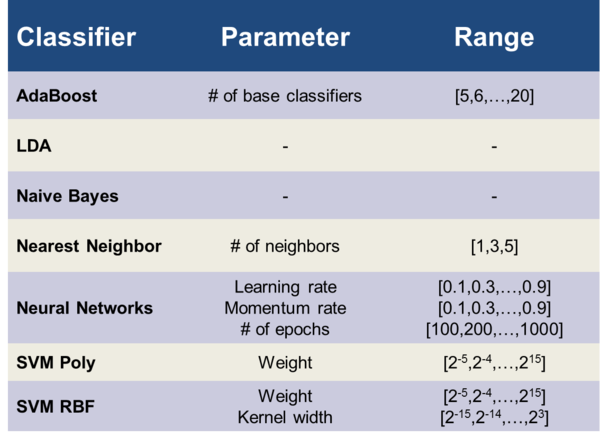
Table 2: Range of the different free parameters of the corresponding classifiers.

 

Leave-One-Out Cross-Validation

In order to test the generalisability and to reduce a possible bias towards higher classification rates by over-fitting, all listed results of the automatic classifiers were generated by performing a leave-one-out cross-validation (LOO-CV). Figure 3 provides a diagram for the used setup. The output of this algorithm is the LOO-CV classification accuracy for every feature set. For the classification of our subsets SUB44 and SUB32, we had 62 different feature sets. The algorithm consequently outputs one LOO-CV classification accuracy, which was optimized with regard to the free parameters of the respective classifier for each of the 62 feature sets.

 

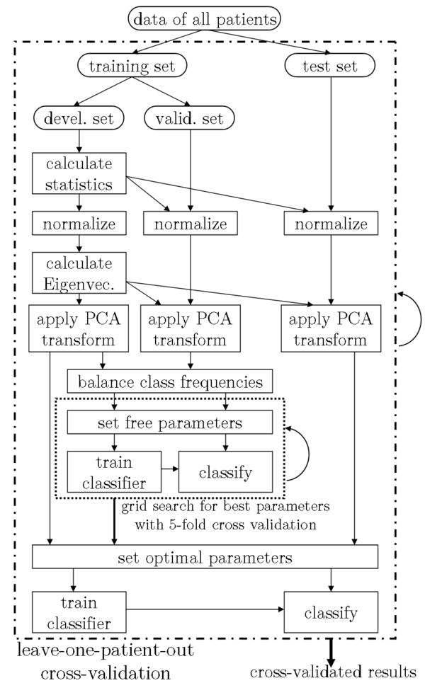
Figure 3: The setup of our experiments, incorporating a grid search for the best classifier parameters and a leave-one-patient-out cross validation. For the grid search, the training set was further subdivided into development and validation set. The parameters for the normalization and the PCA were learned from the development set only.

 

Results

Imaging Modalities

This section focuses on the differentiation of the classification results for feature sets derived from the different modalities. Table 3 lists the results for the 2-class problem and automatic classifiers, Table 4 the results for the 4-class problem.

For all automatic classifiers, the maximum classification accuracies of the available features sets are listed, separated by imaging modality. All values reflect LOO-CV results and were tested for statistical significance with Cohen's Kappa: Parentheses denote results that are not significantly better than random prediction.

The classifications for feature sets from T1-, T2-MRI, PET and Multimodality (combining the three previously named) were carried out on patient subsets SUB44 (2-class) and SUB32 (4-class). The classification for ADC-MRI (SUB22, 22 patients) and X-ray CT (SUB14, 14 patients) was only done for 2-classes, due to the limited dataset number in these groups.

Please note that the results for the PET are based on the SUV normalized datasets since this technique is the standard in nuclear medicine.

 

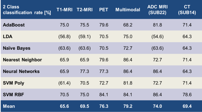
Table 3: Correct classification rates for the differentiation of the low- /high- grade classes. Brackets () indicate non-significant results

 

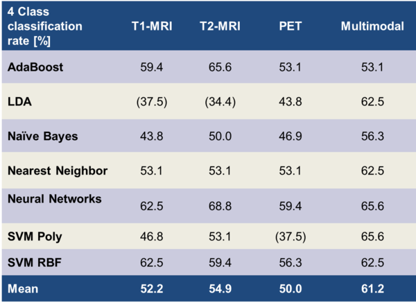
Table 4: Correct classification rates for the differentiation of the four individual WHO grades. Brackets () indicate non-significant results.

 

Discussion

 

Accuracy of Classification for Different Imaging Modalities

It was indicated from the literature that the modalities that we used provide different amounts of information for revealing the underlying tumour grade. For analyzing this, we evaluated classification rates from each modality specifically. We found distinct differences in the classification rates of the imaging modalities, for 2 as well as for 4 tumour classes.

 

2 Classes

Table 3 lists the means and the maxima of the achieved classification accuracies over all classifiers: We found the multimodal approach (86.4%) to be superior to PET (84.1%) and T2- (77.3%), and T1-MRI (75%). In the following, our results are compared to the state of the art from the literature:

Our MRI only based classification rates are higher than those reported by Haegler et al. (8). They performed a manual grading by consensus of two medical experts and achieved an accuracy of 64.9% on 37 patients with pre- & post-contrast T1-, T2-FLAIR-, and proton density MRI. In a study of Riemann et al. (9), a relatively high classification accuracy of 88% is reported for a visual assessment on pre- and post-contrast T1- and T2-MRI images. Their high accuracy for separating low and high tumour grades might be explained by the lack of WHO3 tumours in their patient population (24 WHO1+WHO2, 0 WHO3, 24 WHO4). In a large study (160 patients) Law et al. (10) report an accuracy of 70.6% on grading by consensus of two medical experts on pre- and post-contrast T1- and T2-FLAIR-MRI. In a study with automatic classifiers on MRI data, Zacharaki et al. achieved 87.8% accuracy for 98 patients (11) and reported 94.5% accuracy for the same 2-class problem in a later publication (12). There were some differences in comparison to our studies: First of all, our patient population is more heterogeneous with regard to the imaging parameters, e.g. 1 MRI system and 3 sequence variants vs. 6 systems and 28 sequence variants in our setup. Additionally, their approach relied on 4 different manually defined VOIs covering various regions of the same tumour (enhancing, non-enhancing, necrotic, oedematous), as opposed to only 1 VOI covering the whole tumour in our case. This might introduce a significant amount of prior knowledge when compared to our approach. Li et al. (13) report on 2-classes an accuracy of 89% with a SVM classifier for 154 patients. On the contrary to our study, their features were manually extracted, as medical experts had to rate e.g. the amount and heterogeneity of contrast agent, the amount of haemorrhage or the amount of necrosis.

For PET, various reports for the accuracy of differentiation between low- and high-grade gliomas exist: Pöpperl et al. report a rather high accuracy of 96% for a ROC analysis (AUC 0.967) based on dynamic PET of 54 patients (14). So far, other groups were unable to reproduce these results with their patient populations even if using the same methods. Our lower classification results might also be due to the fact that the PET images for our patient population stem from 2 different PET scanners using 3 different image reconstruction methods, compared to 1 system and 1 reconstruction method. Even though the calibration methods that we applied should have prevented significant inter-device deviations, these methods might not be sufficient.

A recent study on a large patient population (n=143) of Rapp et al. (15) achieved 74% accuracy for a ROC analysis (AUC 0.77) on dynamic PET data, which is slightly less compared to our results.

Even though the heterogeneity of study setups and patient populations make it hard to compare the achieved classification rates, the results from our own methods and those from the literature emphasize that PET is superior to MRI modalities in differentiating low-grade and high-grade tumours.

For the multimodal approach, we find that a combination of features from PET and MRI leads to higher classification rates than features from single modalities. To the best of our knowledge, no systematic study in literature exists on the classification accuracy of the exactly same multimodal features. On a similar note, Floeth et al. (16) assess increased diagnostic abilities of the multimodal (PET+MRI) approach over single modalities for the differentiation of brain tumours and non-neoplastic lesions. Similar results were reported from Pauleit et al. (17), which confirm an increased accuracy of the multimodal approach.

 

4 Classes

Compared to the 2-class problem, the order for the achieved mean classification rates of the 4-class task differed: T1-MRI: 52.5%, T2-MRI: 54.9%, PET: 50.0%, Multimodality: 61.2%. PET was no longer superior compared to the MRI modalities. The classification rates of the single modalities were very similar to each other. Still, we found features derived from multiple modalities to achieve better classification rates. Our highest classification rate for differentiating the 4 WHO grades was 68.8%.

To the best of our knowledge, results in literature for differentiating each of the four WHO grades on basis of medical imaging are still lacking. For reference, we report results on similar topics: Zacharaki et al. (11) achieved an accuracy of 63% for differentiating WHO2, WHO3, WHO4, and metastases of other tumours on 98 patients. They derived features from 4 manually defined VOIs from MRI and classified using support vector machines. In a later publication of the same group (12), they were able to improve their classification rates on the same task to 76.3% by feature selection with a wrapper and the best first search strategy. When comparing to our study, some differences arise: They used unbalanced classes with 22 WHO2, 18 WHO3, 34 WHO4 and 24 cases of metastases of other tumours, whereas we had a smaller patient population with balanced classes. Additionally, the previously listed differences still apply: They had a more homogenous study setup in terms of imaging modalities and probably introduced more prior knowledge by defining manual VOIs covering multiple tumours aspects.

 

ADC MRI & CT

Our results for diffusion-based (ADC) MRI and X-ray CT were derived from smaller subsets of our patient collective (ADC-MRI: 22 patients, CT: 14 patients) when compared to T1-MRI, T2-MRI and PET (44 patients). ADC-MRI achieved a highest classification rate of 86.4%, CT of 78.6%. Due to the limited patient number, results for 4 class classification were not calculated and the accuracies should not be compared to the classification rates of the other modalities.

Our results indicate that the classification rates for these modalities were significantly better than random prediction: An information of the tumour grade can be automatically derived from diffusion MRI and X-ray CT. Especially the high classification rates for ADC-MRI indicate the potential of this modality.

Our findings are supported by several studies from literature: For diffusion MRI, Arvinda et al. (18) report a ROC analysis with an accuracy of 88.2% on 51 patients with low- and high-grade gliomas. They achieve even better results (94% accuracy) for the classification based on the relative cerebral blood volume (rCBV), which was not available for our patients. On the same topic, Hilario et al. (19) reached an accuracy of 88.8% for a ROC analysis of ADC features and 85.6% for rCBV features of 162 patients.

 

Limitations

One limitation of our study was the lesser number of patient datasets which we had available for analysis. The requirements for this kind of study are high: No prior treatment is allowed, a bioptically confirmed tumour is mandatory, and dynamic PET and various MRI sequences need to be acquired. For our patient population, gathering the data was a process of several years. Nevertheless, studies with larger patient populations in all subgroups would be beneficial. A larger patient collection than ours is especially necessary for the differentiation of the 4 WHO grades and the evaluation of the potential benefit of diffusion weighted MRI and X-ray CT.

The achieved maximum classification performance of 90.9% for the differentiation of low and high tumour grades and 68.8% for the 4 WHO grades could be improved. We found a considerable amount of misclassification between the groups WHO2/WHO3 and WHO3/WHO4 (Table 5).

 

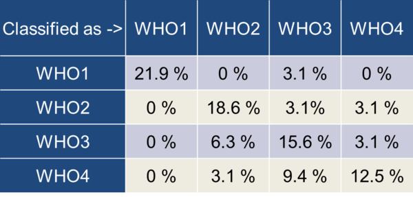
Table 5: Confusion matrix for the highest achieved 4-class classification

 

When comparing the classification results based on medical image data to the tumour grades diagnosed by histology, one has to keep in mind that histological grades represent the tumour in the exact area where the biopsy was taken. It is well known that gliomas should be seen as heterogeneous formations which incorporate regions with varying tumour grade. Additionally, the inter-rater variability in the process of histological grading is not negligible. It is reported to be as high as 20% for glial tumours (20). This variability could be reduced by a consensus agreement of independent histopathologic examinations of multiple experts.

Summary

We presented methodologies and techniques that show that an automatic classification of cerebral gliomas is feasible. Furthermore, our classification results were in line with those provided in literature, which is noteworthy when one takes into account our heterogeneous study setup. It should be noted that this heterogeneity reflects the true clinical case.

As expected, the two-class differentiation of low and high tumour grades achieved better classification results compared to the differentiation of the 4 individual WHO grades. Nevertheless, our results underline that the differentiation of the 4 WHO grades is feasible within certain limitations. Especially the WHO grades 3/4 and 2/3 had a significant overlap in our study.

When it comes to the value of the single modalities in differentiating between low and high-grade tumours, PET using FET as a tracer offers the most valuable information among the presented modalities. This benefit was lost for the 4-class differentiation, where MRI offered better classification accuracies.

In general, the multimodal approach with combined features from MRI and PET offers the best overall classification results. This is comparable with the clinical routine where examinations from nuclear medicine (PET) and radiology (MRI) are performed separately but interpreted in conjunction.

Within the limitations of our study, namely a low number of datasets, diffusion-weighted MRI and CT offer potentially beneficial information on the tumour grade.

In general, for 2 classes as well as for 4 classes, the C-SVM classifier with radial basis function or neural networks in the form of multilayer perceptron are recommendable. For complex problems in this field (class number >2), the k-nearest neighbour classifier is a promising alternative to the aforementioned methods: It features an easy application with only 1 free parameter and fast computation. However, one has to keep in mind that the classification performance of this classifier might be limited for problems with higher dimensionality than ours (maximum of 62 dimensions).

Future Work & Outlook

With the advent of combined PET & MRI scanners (21), the incorporation of multimodal features for the differentiation between tumour types and grades will become easier. Not only is the number of examinations reduced, but the synergistic effects of the system can also be exploited. Furthermore, motion correction of the PET acquisition with the help of MRI is seen as one of the hot topics in the field of MR-PET (22, 23). Additional work should be carried out for incorporating diffusion-, perfusion-weighted, and spectroscopic MRI into a multimodal classification scheme. The accuracy for the differentiation of tumour grades from our own work as well as from literature (24) promise improved diagnostic abilities of such a setup, especially when using MRI spectroscopy. A combined MR-PET scanner could facilitate such acquisitions (25): Dynamic FET-PET must be acquired over a lengthy time period, leaving plenty of time for sophisticated MRI sequences beyond simple T1-, or T2- weighting.

Results from literature (11, 12) indicate that more sophisticated feature reduction and selection approaches, like recursive feature elimination or sequential forward selection, could lead to improved classification accuracy and clarify the varying importance of the individual features on the classification process.

When comparing our results to the literature, we noticed a high heterogeneity in study setups and patient databases. A freely-accessible glioma database featuring imaging data from PET and MRI should be established; as such an initiative could greatly aid future research.

The field of computer aided diagnoses (CAD), which we consider this work to be a part of, is emerging as it proves its value and abilities in a growing field of applications. CAD will not replace the need for well-educated physicians, but will support their work by gathering and summarizing information from multimodal imaging data, helping to provide more accurate diagnoses, and reducing the time required to produce them.

 

References:

 

1.         Weller M. Interdisziplinäre S 2 Leitlinie für die Diagnostik und Therapie der Gliome des Erwachsenenalters. Deutsche Krebsgesellschaft; 2004.

 

2.         Sawin M.D PD, Hitchon M.D PW, Follett M.D PDKA, Torner Ph.D JC. Computed Imaging-Assisted Stereotactic Brain Biopsy: A Risk Analysis of 225 Consecutive Cases. Surg Neurol. 1998;49(6):640-649.

 

3.         McGirt MJ, Woodworth GF, Coon AL, et al. Independent predictors of morbidity after image-guided stereotactic brain biopsy: a risk assessment of 270 cases. J Neurosurg. 2013/05/21 2005;102(5):897-901.

 

4.         Hahn DA, Daum V, Hornegger J. Automatic Parameter Selection for Multimodal Image Registration. Medical Imaging, IEEE Transactions on.29(5):1140-1155.

 

5.         Ritt P, Hahn D, Hornegger J, Ganslandt O, Doerfler A, Kuwert T. Anatomische Genauigkeit der retrospektiven, automatischen und starren Bildregistrierung zwischen kranialer FET-PET und MRT. Deutsche Gesellschaft für Nuklearmedizin (48. Jahrestagung der Deutschen Gesellschaft für Nuklearmedizin). Leipzig; 2010.

 

6.         Haralick R, Shanmugam K, Dinstein I. Textural Features for Image Classification. IEEE Transactions on Systems, Man, and Cybernetics. 1973:610-621.

 

7.         Pearson K. On lines and planes of closest fit to systems of points in space. Philosophical Magazine. 1901;2(6):559-572.

 

8.         Haegler K, Wiesmann M, Böhm C, et al. New similarity search based glioma grading. Neuroradiology.54(8):829-837.

 

9.         Riemann B, Papke K, Hoess N, et al. Noninvasive Grading of Untreated Gliomas: A Comparative Study of MR Imaging and 3-(Iodine 123)-L-α-methyltyrosine SPECT1. Radiology. November 1, 2002 2002;225(2):567-574.

 

10.       Law M, Yang S, Wang H, et al. Glioma Grading: Sensitivity, Specificity, and Predictive Values of Perfusion MR Imaging and Proton MR Spectroscopic Imaging Compared with Conventional MR Imaging. American Journal of Neuroradiology. November 1, 2003 2003;24(10):1989-1998.

 

11.       Zacharaki EI, Wang S, Chawla S, et al. Classification of brain tumor type and grade using MRI texture and shape in a machine learning scheme. Magn Reson Med. 2009;62(6):1609-1618.

 

12.       Zacharaki E, Kanas V, Davatzikos C. Investigating machine learning techniques for MRI-based classification of brain neoplasms. International Journal of Computer Assisted Radiology and Surgery. 2011;6(6):821-828.

 

13.       Li G-Z, Yang J, Ye C-Z, Geng D-Y. Degree prediction of malignancy in brain glioma using support vector machines. Comput Biol Med. 2006;36(3):313-325.

 

14.       Pöpperl G, Kreth FW, Herms J, et al. Analysis of 18F-FET PET for Grading of Recurrent Gliomas: Is Evaluation of Uptake Kinetics Superior to Standard Methods? J Nucl Med. March 1, 2006 2006;47(3):393-403.

 

15.       Rapp M, Heinzel A, Galldiks N, et al. Diagnostic Performance of 18F-FET PET in Newly Diagnosed Cerebral Lesions Suggestive of Glioma. J Nucl Med. February 1, 2013;54(2):229-235.

 

16.       Floeth FW, Pauleit D, Wittsack H-J, et al. Multimodal metabolic imaging of cerebral gliomas: positron emission tomography with [18F]fluoroethyl-l-tyrosine and magnetic resonance spectroscopy. J Neurosurg. 2005;102(2):318-327.

 

17.       Pauleit D, Floeth F, Hamacher K, et al. O-(2-[18F]fluoroethyl)-l-tyrosine PET combined with MRI improves the diagnostic assessment of cerebral gliomas. Brain. March 1, 2005 2005;128(3):678-687.

 

18.       Arvinda HR, Kesavadas C, Sarma PS, et al. Glioma grading: sensitivity, specificity, positive and negative predictive values of diffusion and perfusion imaging. J Neurooncol. 2009;94(1):87-96.

 

19.       Hilario A, Ramos A, Perez-Nunez A, et al. The Added Value of Apparent Diffusion Coefficient to Cerebral Blood Volume in the Preoperative Grading of Diffuse Gliomas. American Journal of Neuroradiology. April 1, 2012;33(4):701-707.

 

20.       Bent M. Interobserver variation of the histopathological diagnosis in clinical trials on glioma: a clinician's perspective. Acta Neuropathol (Berl). 2010;120(3):297-304.

 

21.       Judenhofer MS, Wehrl HF, Newport DF, et al. Simultaneous PET-MRI: a new approach for functional and morphological imaging. Nat Med. 2008;14(4):459-465.

 

22.       Gravel P, Verhaeghe J, Reader AJ. 3D PET image reconstruction including both motion correction and registration directly into an MR or stereotaxic spatial atlas. Phys Med Biol. 2013;58(1):105.

 

23.       Ouyang J, Li Q, El Fakhri G. Magnetic Resonance-Based Motion Correction for Positron Emission Tomography Imaging. Semin Nucl Med. 2013;43(1):60-67.

 

24.       Beppu T, Sasaki M, Kudo K, et al. Prediction of malignancy grading using computed tomography perfusion imaging in nonenhancing supratentorial gliomas. J Neurooncol. 2011;103(3):619-627.

 

25.       Neuner I, Kaffanke J, Langen K-J, et al. Multimodal imaging utilising integrated MR-PET for human brain tumour assessment. Eur Radiol. 2012;22(12):2568-2580.