
This section contains excerpts from the following publication:
Ritt, Philipp; Kuwert, Torsten; Quantitative SPECT/CT; Molecular Imaging in Oncology Recent Results in Cancer Research, Springer Berlin Heidelberg Berlin, pp. 313-330, 2013
Ritt, Philipp; Vija, Hans; Hornegger, Joachim; Kuwert, Torsten; Absolute quantification in SPECT; European Journal of Nuclear Medicine and Molecular Imaging, vol. 38, pp. 69-77, 2011
Motivation
Single-photon emission computed tomography (SPECT) and PET allow the visualization of the distribution of radioactivity within the human body. Both modalities are widely used for clinical purposes. SPECT and PET also promise to exactly quantify the concentration of radioactivity within a given volume of tissue in absolute units, e.g. as kilobecquerels per cubic centimeter. This process is compromised by photon scatter, photon attenuation and partial volume artifacts.
In PET, options to correct for these confounding variables have been developed and validated several decades ago, owing to the technical advantages offered by positron decay and coincidence detection. In SPECT, technical progress in that regard has been considerably slower with various reports emphasizing the lack of quantitative abilities.
For orientation, a simplified diagram of the image formation chain for quantitative PET and SPECT is given in Figure 1.
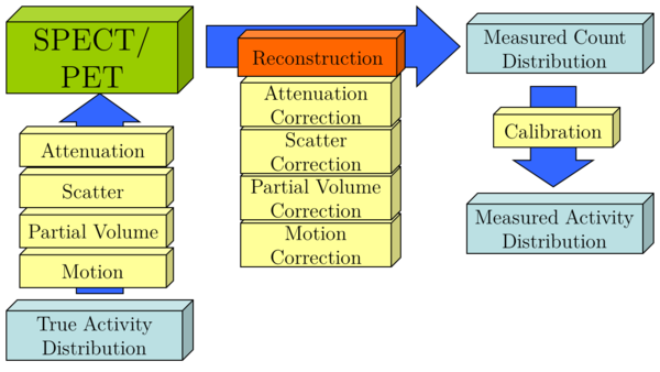
Figure 1: Schematic of image formation chain of SPECT and PET
We will now shortly introduce the effects of attenuation, scatter, and partial volume with a short explanation of the underlying effect and examples of correction techniques. In addition, we will briefly outline a calibration technique. We will conclude with a discussion of the potential of SPECT and PET quantification for clinical applications and present some validation studies.
Attenuation Correction in ECT
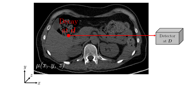
Figure 2: Schematic diagram of photon attenuation for SPECT
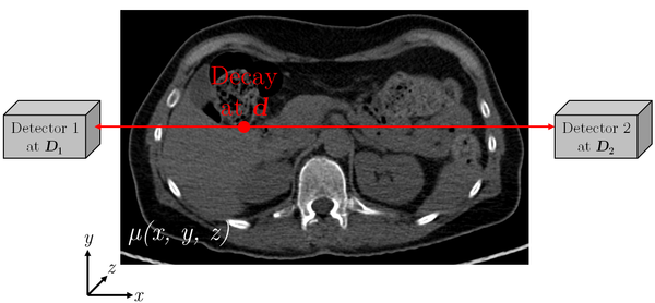
Figure 3: Schematic diagram of photon attenuation for PET
ECT images are affected by attenuation artifacts. In the case of SPECT imaging, the probability $P_{\operatorname{Det}}$ that a gamma quantum emitted at position $\vec{d} \in \mathbb{R}^{3}$ (see Figure 2) reaches the detector at position $\vec{D} \in \mathbb{R}^{3}$ (assumed that it is emitted in the proper direction) is calculated according to Equation 1:
$$P_{\operatorname{Det}}\propto \int_{C}{-\mu(x,y,z)\,\mathrm{d}s} \qquad \text{Eq. 1}$$
with the two endpoints of the path $C$ given by $\vec{D}$ and $\vec{d}$ .
$$P_{\operatorname{Det}}\propto \int_{C}{-\mu(x,y,z)\,\mathrm{d}s} \qquad \text{Eq. 2}$$
with the two endpoints of the path $C$ given by $\vec{D_1}$ and $\vec{D_2}$.
The integral covers essentially the path $C$ (by approximation a straight line) of the radiation from its origin through the object, to the location of detection.
The probability for SPECT consequently depends on the (unknown) location of the decay $\vec{d}$ and on the linear attenuation coefficients $\mu(x,y,z)$ of the object. In contrary, in PET imaging (Figure 3) the probability only depends on the linear attenuation coefficients along the line of response (LOR) $\vec{D_2}-\vec{D_1}$ where the decay happened, but not on the exact location in this LOR (Equation 2).
For the attenuation correction in the reconstruction step, the spatial distribution of the attenuation coefficients of the examined object for the photon energy of the radionuclide used needs to be known. Several methods for obtaining attenuation maps have been employed so far:
The maps can be estimated, if the contours of the object (e.g. via rough segmentation of the SPECT or PET image) and the attenuation coefficients are known (e.g. attenuation coefficient of water). The object can be assumed to be homogeneous with regard to this coefficient (Chang's correction). This method is still applied very successfully to SPECT imaging of the brain, where only one class is predominant (soft brain tissue). However, it is not very accurate for ECT imaging of the thorax or pelvis, where large amount of other tissues (e.g. lung and bone) are present.
Another way of generating the attenuation maps is through a simple transformation of a transmission scan. The transmission images need to be converted to attenuation factors at the effective energy of the emission scan (140 keV for Tc-99m, 511 keV for PET) and corrected for the spatial registration between the emission and transmission images. This conversion is often characterized by a bi-linear transformation, which is displayed in Figure 4:
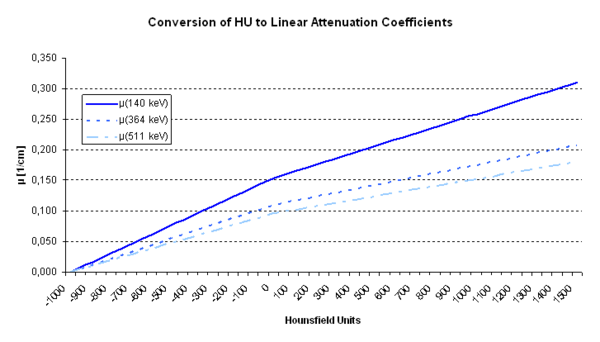
Figure 4: Conversion from Hounsfield Units to Linear Attenuation Coefficients for different photon energies
The resulting attenuation map can be easily integrated into common iterative reconstruction techniques. See Figure 5 for a side-by-side comparison of non-attenuation corrected and attenuation corrected SPECT images of a homogenously filled phantom.
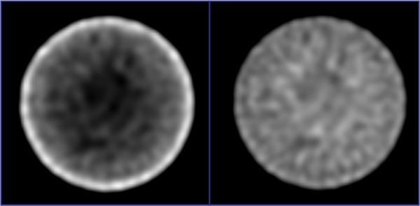
Figure 5: Side-by-side comparison of (left) non-attenuation and (right) attenuation corrected SPECT phantom images
Scatter
The simple reconstruction techniques in earlier methods neglected the cross talk between the individual lines of response. This assumption fails if photon scatter occurs. Scatter correction is another important requirement for (quantitative) ECT imaging. Scattered radiation is produced when gamma quanta emitted from decaying nuclei interact with surrounding atoms. Compton scattering is the prevalent scatter process in the energy range of clinically-utilized radio-tracers.
The energy $E_{\operatorname{S}}$ of the scattered photon depends only on the scattering angle $\phi$ and is given by Equation 3, where $E_0$ is the energy of the photon before the scattering and $m_{e}c^2$ the invariant mass of the electron. The energy transfer thus does not depend on the density or atomic number of the absorbing material. However, the total probability that a photon is scattered by this effect depends heavily on the properties of the absorbing material, most importantly the electron density.
As seen in Equation 3, the gamma quanta loose energy and change their momentum and direction in the scatter process. Because of the intrinsic energy resolution of the detector, the system cannot discriminate between unscattered quanta and quanta that have lost a small amount of energy in the scatter process. As a consequence some scatter is allowed in the image formation.
$$E_{\operatorname{S}} = \dfrac{E_0}{1+\frac{E_o}{m_{e}c^2}(1-\cos(\phi))} \qquad \text{Eq. 3}$$
In simple FBP, it is assumed that the decay took place exactly perpendicular to the detection plane and the detection location (for SPECT, under assumption of parallel-hole collimation). For scattered quanta, because of the change in direction in the scatter process, not only the distance of the radionuclei along the LOR is unknown, but also the correct positions of the LOR to the radionuclei. However, not all information about the originating nuclei is lost. Scattered radiation is therefore often understood as anisotropic noise that reduces the image quality of an ECT image.
There exist a variety of methods to correct for scattered radiation. Some of them rely on “passive” methods: For example, the camera's energy window could be narrowed or the lower discriminator cut-off of the window could be increased in order to avoid accepting scattered photons. A significant drawback of this method is that unscattered photons are also rejected due to the limited energy resolution of the gamma camera. Even with a relatively small energy window of $\pm$ 5 keV for Tc-99m (140 keV), on basis of Equation 3, photons with scatter angles of up to 30 degrees are still accepted.
More common approaches utilize dual-, triple-, or even multi-energy windows. The additional scatter energy windows are placed below or above the photopeak energy window (Figure 6); the scatter images are acquired simultaneously with the photopeak image.
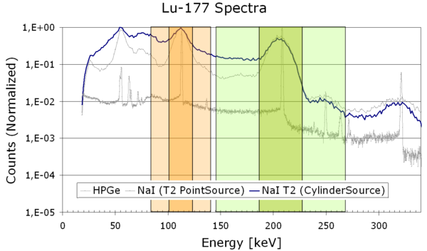
Figure 6: Energy window diagram featuring two photopeak windows (dark orange, dark green) and their corresponding scatter windows (light colors)
For each pixel of the projection image, the amount of scattered radiation in the photo peak window image is estimated from the scatter window images. Subsequently, this amount can be subtracted from the projections or incorporated in the iterative reconstruction.
Partial Volume Effects
Partial volume effects are caused by the limited spatial resolution of emission tomography devices. Region of interest (ROI) in structures with heterogeneous activity distribution below approx. two-times the FWHM of the spatial resolution are degraded. The activity is either under- or over-estimated, depending on the combination of “spill-in” and “spill-out” effects. Spill-in refers to the effect that activity from outside the ROI or structure due to the limited spatial resolution is integrated into the ROI: The activity inside the ROI is increased. Spill-out is understood as the activity of the ROI/structure which is distributed over the borders (again due to the limited spatial resolution) and therefore “lost” for the quantification of that structure: the activity inside the ROI is decreased.
The degree of the partial volume effect depends on the (spatially varying) system resolution of the imaging system, the patient (e.g. motion), and the true distribution of radioactivity in the image.
In SPECT systems, the spatial resolution (which, in the following, is understood as the FWHM of a point source) is limited mainly by the collimator performance. Unlike PET, SPECT utilizes absorptive collimation to identify the direction of the photon LOR. Only a small fraction of the gamma quanta that hit the collimator surface pass through it. This leads to heavily limited detection efficiency when compared to PET. Since there is a trade-off between spatial resolution and detection efficiency, SPECT collimators are typically designed with the maximum allowable resolution in order to partially compensate the limited detection efficiency.
Besides the collimator design and geometry, the achievable spatial resolution is also influenced by the detector intrinsic resolution (the spatial resolution of the detector itself, without a collimator). Today, most SPECT detectors are made of a single crystal plate of NaI that illuminates an array of photomultipliers. The intrinsic resolution of the detector is influenced by the photo-peak energy of the imaged radionuclide and the crystal thickness. Higher gamma quantum energy leads to better intrinsic resolution, due to a higher scintillation light output. A larger crystal thickness increases intrinsic resolution, due to the broader spread of the scintillation light before it exits the crystal.
Clinical SPECT detectors typically possess an intrinsic spatial resolution in the range of 3-5 mm for Tc-99m. However, the image resolution for the SPECT system depends highly on the collimator design and the source-to-collimator distance. For parallel-hole collimation of Tc-99m and typical source-to-collimator distances it commonly ranges from 7 to 15 mm FWHM, which is considerably higher than that seen in PET (2-5 mm FWHM). By applying other collimator geometries, e.g. (multi-)pinhole, even lower spatial resolution than in PET can be achieved. However those collimator geometries are more frequently for small animal studies than in clinical practice.
For clinical PET, the achievable spatial resolution mainly depends on the size of the individual crystal elements and the detector block geometry (e.g. size of the gantry bore). Ultimately, the PET resolution is limited by the positron's free path length in between the initial decay and the annihilation (which is what is detected in PET). Another factor is the acollinearity of the two coincident gamma quanta: The remainder of the kinetic energy of the positron at the point of annihilation causes the two emitted gamma quanta to not be exactly emitted in a perpendicular direction (180°) but in smaller angles. These effects sum up to physical limits of ~2 mm for a clinical PET system.
Calibration
A calibration of the SPECT imaging system volume sensitivity $S_{\operatorname{Vol}}$ (Equation 4) is the final requirement for absolute quantitative imaging. This is typically obtained by a correlation of the results to a calibrated well counter. The principle is briefly outlined in this section, details can be found for example in the NEMA protocols. In order to avoid partial volume effects, a large cylindrical phantom with known activity concentration $c_{\operatorname{Vol}}$ is scanned. Corrections for attenuated and scattered photons are applied in the reconstruction. A large VOI with volume $V_{\operatorname{VOI}}$ is placed on the reconstructed image. $T_0$ is the start time, $T_{\operatorname{acq}}$ the duration of the acquisition. $T_{\frac{1}{2}}$ is the half-life of the used radionuclide and $T_{\operatorname{cal}}$ the time of the activity calibration. $R$ represents the counting rate measured in the VOI. Finally, according to Equation 4, a calibration factor from the detected counts per second to Becquerel is derived. In the equation, the measured count rate $R$ is normalized by the volume $V_{\operatorname{VOI}}$ and the activity concentration $c_{\operatorname{Vol}}$. The other factors of the equation account for the differences between aforementioned time points.
$$ S_{\operatorname{Vol}} = \dfrac{R}{V_{\operatorname{VOI}} \cdot c_{\operatorname{Vol}}} \cdot \exp\left(\dfrac{T_0 - T_{\operatorname{cal}}}{T_{\frac{1}{2}}} \cdot \ln 2 \right) \cdot \left(\dfrac{T_{\operatorname{acq}}}{T_{\frac{1}{2}}}\cdot \ln 2 \right) \cdot \left(1-\exp \left( -\dfrac{T_{\operatorname{acq}}}{T_{\frac{1}{2}}} \cdot \ln 2 \right) \right)^{-1} \qquad \text{Eq. 4}$$
The calibration factor is specific for every radio nuclide as to different intrinsic detector sensitivities and collimators used. Due to non-linearities of the detector at different count rates and dead time effects at high activities, count rate-dependent calibration factors for the same radionuclide should be applied as well. Most notably those effects are more pronounced for high energy radionuclides.
For PET imaging, this step is often automated and included in the daily quality control procedure. A homogenous Ge-68/Ga-68 phantom with known activity is placed in the PET field of view and data is acquired over a certain period of time. Subsequently, a calibration factor is calculated, stored, and automatically applied to the reconstructed PET data. However, to achieve more accurate values, a cross calibration between the well counter and the system, analogously to the above listed SPECT procedure is recommended.
Results
A survey of the current literature as well as our own work show that ECT can be quantitative with errors below 10%, even in a clinical environment (Figure 7).
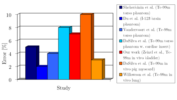
Figure 7: Reported quantitative errors from various phantom and in-vivo studies
To achieve this, a careful setup and calibration of a state of the art SPECT/CT or PET/CT system is required. Equally important is an iterative reconstruction software which is able to model the imaging physics and to correct for degrading factors. Due to the higher spatial resolution of the clinically PET systems and the reduced partial volume effects, PET can reach a better quantitative accuracy for smaller structures than SPECT.