
Contact

 +49-9131-85-27775
 +49-9131-85-27270
Secretary
| Monday | 8:00 - 12:15 |
| Tuesday | 8:00 - 16:45 |
| Wednesday | 8:00 - 16:45 |
| Thursday | 8:00 - 16:45 |
| Friday | 8:00 - 12:15 |
Address
Friedrich-Alexander-Universität Erlangen-Nürnberg (FAU)
Lehrstuhl für Informatik 5 (Mustererkennung)
Martensstr. 3
91058 Erlangen
Germany
Lehrstuhl für Informatik 5 (Mustererkennung)
Martensstr. 3
91058 Erlangen
Germany
Powered by

Epipolar Consistency
Contact: Andre Aichert
Table of Contents
1 About this page
Epipolar Consistency has been shown to be a powerful tool in calibration and motion correction for flat panel detector CT (FD-CT) and other X-ray based applications. The epipolar consistency conditions (ECC) apply to projection data directly and can be used to correct for 3D parameters without 3D reconstruction. The computation of an epipolar consistency metric is real-time capable for small sets of images and can be parallelized for large sets of images. This document briefly describes an algorithm to compute a metric for the epipolar consistency conditions (ECC) between to X-ray images. We assume that the reader is familiar with epipolar geometry [4] and has basic knowledge of X-ray physics and the Radon transform [3]. We will briefly describe an improved version of the algorithm presented by Aichert et al. [1].
2 Data
Let
and
denote two X-ray projections with known projection matrices
and finite source positions
and
accordingly, where
denotes equality up to positive scalar multiples. Let
be two lines in real projective two-space of the image
and
, respectively. Then they are corresponding epipolar lines if there exists an epipolar plane
with
where
denotes the pseudo-inverse. An epipolar plane is any plane which contains both source positions
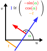
A line
can be characterized as the set of solution to the homogeneous equation
or by its angle
and signed distance to the origin
Every pixel in these images represents an X-ray intensity, which can be transformed into an integral over absorption coefficients
where
is the function of X-ray absorption along the backprojection ray of the pixel
with a distance to the source
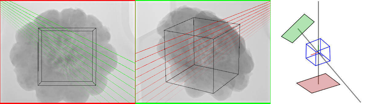
. Please see Figure 1↑, left, center, for two example X-ray images before preprocessing with several exemplary epipolar lines. Further, let
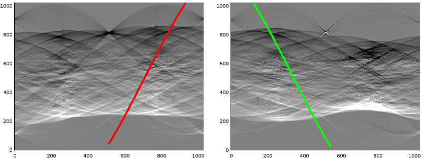
denote the Radon transform of the thus transformed image
with
compare Figure 2↑. See Figure 3↓ for radon derivatives of the pre-processed images from Figure 1↑. Note that a line bundle forms a sinusoid curve in Radon space.
3 Epipolar Consistency
The epipolar consistency conditions state that the derivative in orthogonal direction of the integral along an epipolar line is redundant with the same of the corresponding epipolar line in the other image
where
denotes the Radon transform of the image
and
is its derivative, with
and the symmetry
Since all epipolar lines intersect in the epipole, we have a one-parameter family of lines in each image with 1-1 correspondences. The lines are related via their epipolar planes, which in turn form a pencil of planes. Our goal is to parametrize the pencil of epipolar planes
with a single angle
. Using the relationship between epipolar lines and planes, we can define a metric for consistency between two images as the integral over the plane angle
Since all epipolar planes must contain the line connecting the two source positions
, we compute the consistency metric numerically as follows:
- Use the plane through the center of the object as a reference plane for
- Find a sufficiently small differential angle (not discussed here)
-
Iterate over
from
to
and compute
by rotation about the line connecting
- Compute
- Compute
- Sum over all
A large portion of the algorithm discussed in the previous section is linear. Our goal is to write it as a matrix multiplication by the vector
.
4 Implementation
4.1 Plücker-Matrices
This section assumes basic knowledge of about lines in two- and three-space. The baseline
is the line in three-space connecting the two source positions
. We express the line as an anti-symmetric matrix.
The anti-symmetric Plücker matrix is defined as
where
defined by the six distinct elements
They always fullfill the Grassmann-Plücker relation
. These 6 values are also called Plücker coordinates of the line. We recommend the paper by Blinn [2] about the Plücker matrix. Using Plücker coordinates, we can easily express the direction of the line
and the normal to the plane containing the line and passing through the origin
The 2D-equivalent exists as a
Plücker matrix that is related to the cross-product via
where
We can thus write
and we introduce a dual Plücker matrix
Plücker matrices allow us to directly express the common plane of a point
and a line
4.2 ECC algorithm using Plücker coordinates
Assuming that the object is located in the world origin, we can define the reference plane directly
We can also define an orthogonal plane, which contains the baseline
If we assert that the normals of the two planes have unit length, we can thus express any epipolar plane as a linear combination of the two. Specifically, we have
with
. Projection to the two detectors is also a linear operation, so we arrive at the following compact formulation
with
and
. With
and
we have
and
, respectively. The two lines are generally not orthogonal.
5 Octave Source Code
5.1 Loading Data
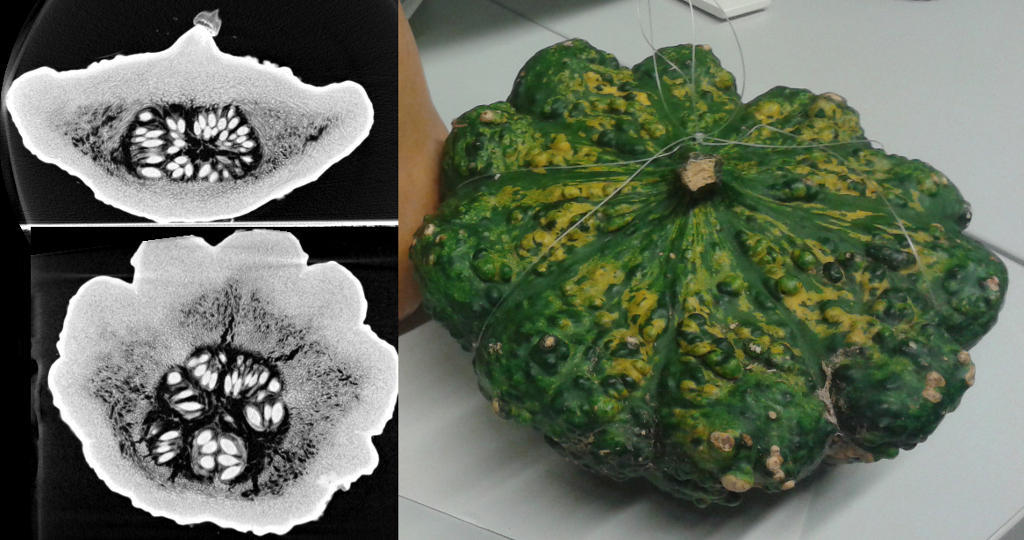
We provide two example data sets. A pumpkin as an example for an organic structure and a toy gun as an example of an artificial structure. We use NRRD as an image format and provide a C++ header-only library to load and save NRRD images. We recommend Fiji/ImageJ as an image viewer. For MATLAB/Octave, there exists a nice function to load NRRD files from Mathworks FileExchange, distributed under its own BSD license. All NRRD files contain a human-readable ASCII header. Our projection images contain a
projection matrix (MATLAB-like format). In addition, there is a comment in the last line with the offset in bytes to the raw float data, followed by an empty line.
NRRD0004 dimension: 2
encoding: raw
endian: little
sizes: 2480 1920
type: float
Projection Matrix:=[...]
# Offset to raw data:      570 bytes.
By convention, we refer to the function
, in words the “derivative in
-direction of the Radon transform” as dtr, compare Figure 3↑. These dtrs have to be pre-computed from the projection images. We recommend to use our minimal working data set to get started quickly. For in-depth investigations, we provide you with two complete data sets of 15 images each, along with a Windows/CUDA binary to compute the Radon transform and tools to convert and edit NRRD files (see Downloads↓ Section). Please see the first lines in ecc_demo.m and adjust the paths to two input images as desired.
5.2 Computing the ECC
The algorithms described in this paper are implemented in the function
% Mapping to epipolar lines
[K0 K1]=ecc_computeK01(P0,P1, n_x, n_y);
Here, P0 and P1 are the projection matrices and n_x and n_y the number of image columns and rows. The corresponding implementation located in the file ecc_demo/ecc_computeK01.m. The sampling of the ECC can be summarized in the following code
consistency=0; % resulting metric
dkappa=0.2*pi/180
for kappa=[-pi*0.5:dkappa:pi*0.5]
x_kappa=[cos(kappa); sin(kappa)];
l0_kappa=K0*x_kappa;
% Sample Radon derivatives at corresponding locations
[v0 x0, y0, w0]=ecc_sample_rda(l0_kappa, rda0, range_t);
[v1 x1, y1, w1]=ecc_sample_rda(l1_kappa, rda1, range_t);
consistency+=(v0-v1)*(v0-v1)*dkappa;
end %
Here, dkappa is arbitrarily chosen to be
. Adjust this value to obtain a dense sampling of lines. The code in ecc_demo.m computes redundant values for both
at the same time and is able to terminate early, when the lines no longer intersect the image. It also contains a lot of code for visualization. A brief version of ECC computation can be found in the file ecc_demo/ecc_compute_consistency.m .
5.3 Heuristic for the sampling distance
The number of samples drawn from the Radon transforms depends linearly on the angular step
. On the one hand, choosing
too small results in slow run-times, on the other hand, choosing
too large results in under-sampling and less accurate ECC values. For best results,
should be chosen as large as possible, while consequent samples drawn from Radon space should be no farther apart than the size of one Radon bin. Let
and
denote the Radon bin size in angular and distance directions respectively. Further, let
and
, respectively, denote the image of the world origin in image 0 and 1. This point serves as a reference point and is thus always located inside the object and close to the center of the image. To find a good heuristic for an appropriate value for
, we want either the angle
or distance
between the epipolar lines
and
to be less than the Radon bin size
where
is the angle between two homogeneous lines and
the euclidian distance between a line and an image point. The same should hold for
,
and
, respectively. Whether
or
is the limiting dimension depends on the location of the epipoles. If they are close to the image, a differential change in
will affect
more than
, and vice versa if the epipoles are far away. One should choose
adaptively for each pair of images.
5.4 Screenshot of the demo
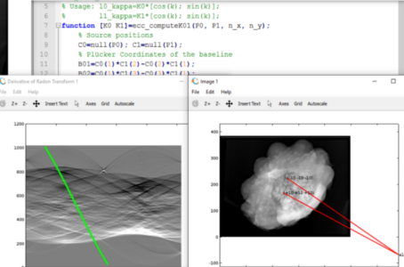
Figure 5 Screenshot of the demo running on windows. (enlarge)
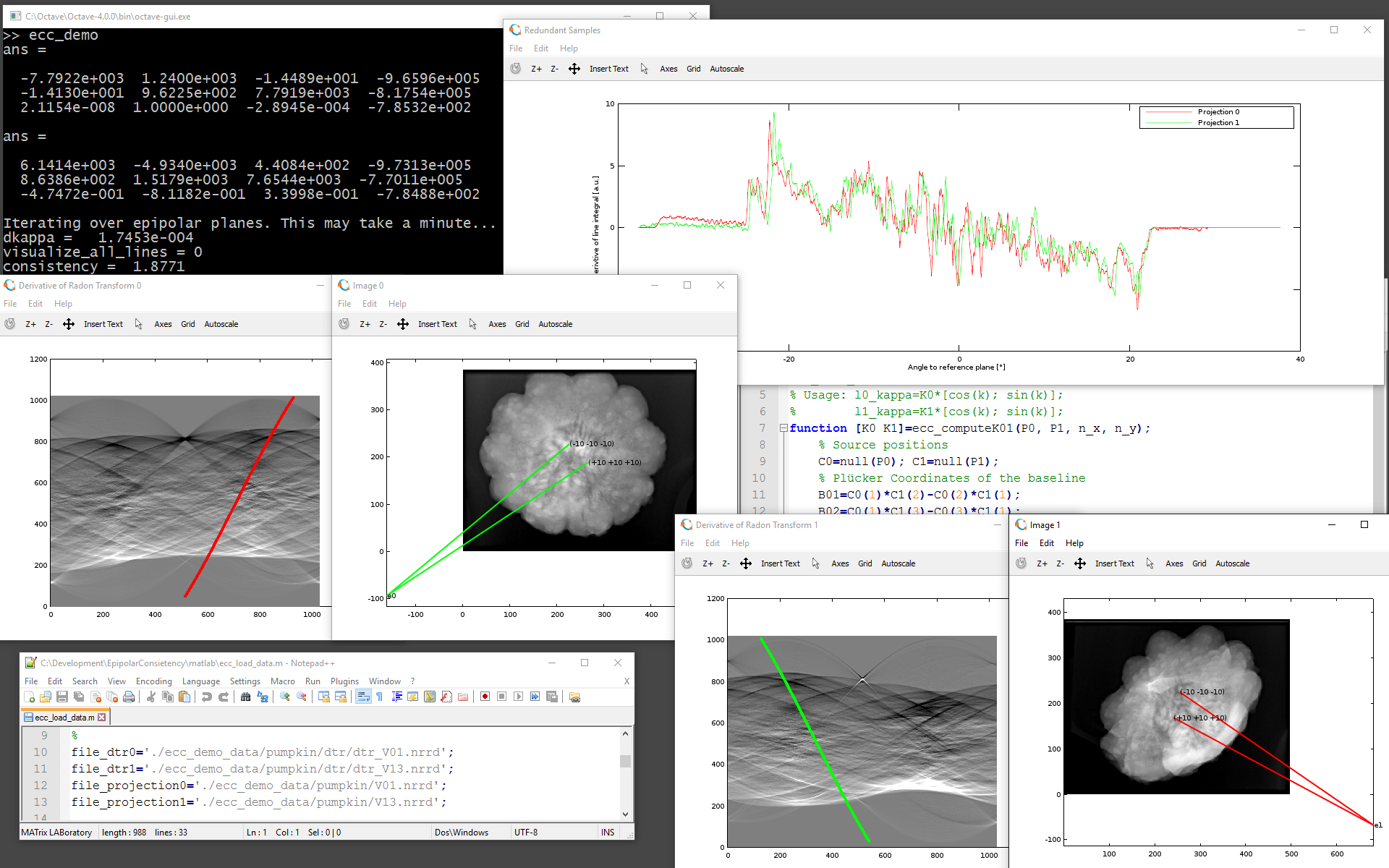
Downloads
- OpenSource c++ library on GitHub
-
Windows binaries for a Demo and tools to view CT trajectories
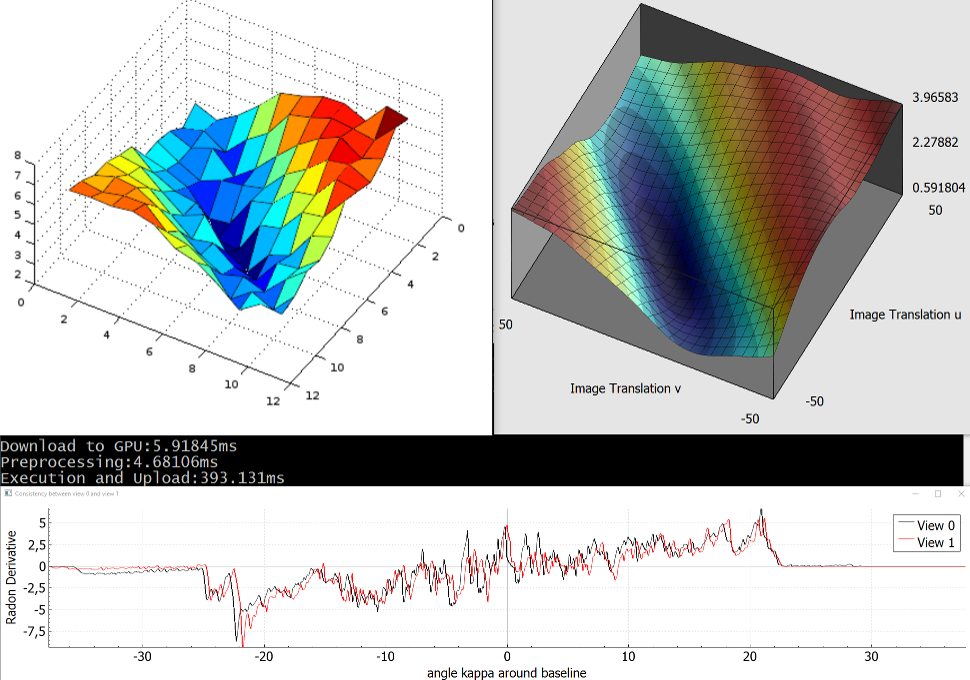
Click here for another screenshot comparing runtimes for this Octave demo and a CUDA implementation of ECC
(1 hour for 11x11 versus 1 second for 501x501, plot shows detector shifts of +/-50 pixels). - Octave and Octave for Windows
- The octave source code including two example images.
- Two example data sets with 15 images each
- Windows binaries for visulaization
References
[1] . Epipolar Consistency in Transmission Imaging. Medical Imaging, IEEE Transactions on, 34(11):2205-2219, 2015.
[2] . A homogeneous formulation for lines in 3 space. ACM SIGGRAPH Computer Graphics, 11(2):237-241, 1977.
[3] . Computed Tomography: From Photon Statistics to Modern Cone-Beam CT. Springer, 2008.
[4] . Multiple View Geometry in Computer Vision. Cambridge University Press, 2004.