


Ordered Subsets
Iterative Reconstruction with Ordered Subsets
This is a short tutorial that describes the ideas of ordered subsets and how this can be implemented in CONRAD. The references to the CONRAD sources implementing this are found at the end of this tutorial.
Gradient Descent Iterative Reconstruction
Besides direct methods like the filtered backprojection, also iterative methods can be used for medical image reconstruction. These methods start with an arbitrary image and in every iteration the reconstructed image is updated such that it converges to the exact reconstruction.
The clear benefit of such algorithms is, that they have an improved insensitivity to noise and they can even create very good solutions for incomplete data.
The minimum of a convex function is found by following the gradient of the function in negative direction.
In the case of image reconstruction (where the solution for the equation AX = P is required), the reconstructed image is computed by the gradient
descent reconstruction method where each update is performed as follows:
- Forward project the current backprojected image X k: AX k
- Subtract the forward projection from the projection P: (P - AX k)
- Backproject the projection difference: multiplication with A T
- Multiply the backprojection with the parameter λ
- Add to the current backprojected image X k
Ordered Subsets Reconstruction
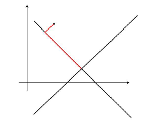
The main disadvantage of iterative reconstruction methods is the higher computational effort compared to direct methods where only one backprojection step is needed for the reconstruction. According to the angle between the projection hyper planes, they can sometimes converge very slow. If two considered hyper planes are orthogonal to each other, the solution is found after at most two iteration steps. The steeper the angle between the hyper planes, the longer it takes for the algorithm to converge. The influence of the angle can be seen in the images 1 and 2. The orthogonal hyper planes in image 1 (in this case the hyper planes are lines) result in a much faster convergence than the hyper planes with a steep angle inbetween in image 2 (Source of image 1 and 2: Slides for "Diagnostic medical image processing", WS 2012/13, Andreas Maier, Joachim Hornegger, Markus Kowarschik). Because of the slow convergence, many techniques were developed to speed the iterative methods up. One of these techniques is the ordered subsets (OSS) reconstruction. For OSS each iteration is not performed for the whole projection, but for subsets of P. This can speed up the convergence by using knowledge of the order of the projection acquisition. This way, subsets of the projection can be chosen, that are more likely to be orthogonal to each other. Because only subsets of the whole projection are considered, the computational effort can be lowered significantly.
 |
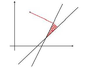 |
| Img 1: Iterative reconstruction orthogonal | Img 2: Iterative reconstruction steep angle |
Ordered Subsets Algorithm in CONRAD
The OSS-classes in CONRAD use the OpenCLGrid-classes and the OpenCL-projection and -backprojection methods. First a 2D- or 3D-phantom is created and projected with the available ProjectRayDrivenCL-methods. The sinogram represents the projection P from which the subsets will be created. In the reconstruct-method an initial reconstructed image img_k is created, that is only filled with zeros. This stands for the starting image X 0. Then the iteration is started with two for-loops going through all iterations and for every iteration considering all subsets. The projection subsets are created in the method getSubset and after the projections are split into the different subsets, the update step is only executed for these subsets. After each update, the subsets are then combined again in the method combiningSubsets. After the last iteration step or if the mean squared error between the prior image X k and the updated image X k+1 is below a threshold, the achieved reconstructed image img_k is returned and shown. The mean squared error is computed after each iteration step in the method mse.
The final code for the OSS reconstruction can be found in the package edu.stanford.rsl.tutorial.fan in the class OSSReconstructionFan (for 2D fan beam geometry) and in the package edu.stanford.rsl.tutorial.cone in the class OSSReconstructionCone (for 3D cone beam geometry).
Copyright by Anja Pohan